Real data: lineage-traced single cells
This tutorial runs TwINFER on single-cell RNA-seq data with clone labels from a lineage-tracing experiment (a barcode, CellTag, LARRY, FateMap, …). Cells that share a label descend from the same labelled cell and form a clone. Unlike the simulated twins of the simulation tutorials, real clones have one to many cells, and many labelled cells are singletons; infer_with_twinfer handles this directly.
The steps are the same for any dataset:
load the expression matrix and the clone label of every cell;
choose the cells of one sample / time point and the genes;
normalise (if the matrix holds raw counts) and build the input table: one row per cell,
clone_id, one column per gene;score the gene pairs: three z-scores, Benjamini-Hochberg correction, inference scenario;
rank the pairs and draw the network.
Several choices depend on the dataset: which columns hold the clone label and the sample, whether the matrix holds raw counts, which cells and genes to use. Each of them is marked Depends on the dataset, followed by what we do for LARRY, the example below.
Example data. The repository ships one dataset, used here: mouse haematopoietic progenitors barcoded with LARRY and sequenced 2, 4 and 6 days later (Weinreb et al., Science 2020), real_data/LSK_d2_d4_d6.h5ad (238 MB, stored with Git LFS: run git lfs pull after cloning if the file is only a small text pointer).
1. Setup and data
Results are written to tutorial_output/real_data_lineage_tracing/, next to this notebook; change output_dir to save them elsewhere. infer_with_twinfer(..., save_to=path) saves its result table (.csv, .csv.gz, .tsv or .parquet) and writes the settings of the call next to it (<name>_settings.json); save_result(table, path) saves any other table the same way.
import warnings
from pathlib import Path

import anndata as ad
import matplotlib.pyplot as plt
import numpy as np
import pandas as pd
import scipy.sparse

from twinfer.inference.covariance_decomposition_z_scores import INFERENCE_SCENARIOS, infer_with_twinfer, save_result
from twinfer.inference.ranked_edges import ranked_edge_lists
from twinfer.plotting.network_plots import network_from_scenarios, plot_grn
from twinfer.utils.paths import get_repo_root

warnings.filterwarnings("ignore", message="Observation names are not unique")   # repeated 10x barcodes, see below
output_dir = get_repo_root() / "tutorials" / "tutorial_output" / "real_data_lineage_tracing"   # where the results are saved (next to this notebook)
adata = ad.read_h5ad(get_repo_root() / "real_data" / "LSK_d2_d4_d6.h5ad")
adata
AnnData object with n_obs × n_vars = 72946 × 25289
    obs: 'Library', 'Time point', 'Starting population', 'Cell type annotation', 'Well', 'SPRING-x', 'SPRING-y', 'clone_id', 'n_genes_by_counts', 'total_counts', 'pct_counts_in_top_50_genes', 'pct_counts_in_top_100_genes', 'pct_counts_in_top_200_genes', 'pct_counts_in_top_500_genes', 'total_counts_mt', 'pct_counts_mt'
    var: 'mt', 'n_cells_by_counts', 'mean_counts', 'pct_dropout_by_counts', 'total_counts'
    uns: 'log1p', 'neighbors', 'pca', 'umap'
    obsm: 'X_pca', 'X_umap'
    varm: 'PCs'
    obsp: 'connectivities', 'distances'
Depends on the dataset. Any AnnData object (or a cells × genes matrix with a table of cell annotations) works. The settings below name the column of adata.obs with the clone label, the value that marks cells without a clone, the column with the sample / time point, and whether X holds raw counts or normalised values.
For LARRY: the clone label is clone_id, cells without a detected barcode have clone_id = -1, the samples are the days in Time point (2, 4, 6), and X is already normalised by the authors (each cell scaled to the same total, then log1p), so it is used as it is.
# ============ depends on the dataset (values for LARRY) ============
clone_column = "clone_id"          # clone label of each cell
unlabelled = -1                    # value of cells without a clone label (None if every cell has one)
sample_column = "Time point"       # sample / time point; each is scored separately
x_is_raw_counts = False            # True: X holds raw counts (normalised below); False: X is already normalised
# =================================================================
Check what X holds before setting x_is_raw_counts: raw counts are whole numbers. For LARRY the values are not whole numbers and are at most about 6 (log scale): already normalised.
sample = adata.X[:1000]
sample = sample.toarray() if scipy.sparse.issparse(sample) else np.asarray(sample)
print("whole numbers only:", bool(np.allclose(sample, np.round(sample))), "| largest value:", float(sample.max()))
whole numbers only: False | largest value: 6.358935832977295
2. Clones per sample
Clones with two or more cells give the twin terms (z_rho_s, z_rho_Delta), from all their within-clone cell pairs, each clone with weight 1. Singletons contribute only to the expression correlation (z_rho). The more clones with two or more cells, the more power.
obs = adata.obs
labelled = (obs[clone_column] != unlabelled) if unlabelled is not None else pd.Series(True, index=obs.index)
rows = []
for value, group in obs[labelled].groupby(sample_column, observed=True):
    sizes = group[clone_column].value_counts()
    rows.append({sample_column: value, "cells with a clone": len(group), "clones": len(sizes),
                 "clones with >= 2 cells": int((sizes >= 2).sum()), "singletons": int((sizes == 1).sum()),
                 "largest clone": int(sizes.max())})
clones_per_sample = pd.DataFrame(rows).set_index(sample_column)
clones_per_sample
| cells with a clone | clones | clones with >= 2 cells | singletons | largest clone | |
|---|---|---|---|---|---|
| Time point | |||||
| 2.0 | 2809 | 1625 | 863 | 762 | 6 |
| 4.0 | 6121 | 2497 | 1674 | 823 | 12 |
| 6.0 | 15978 | 2630 | 2150 | 480 | 50 |
3. Build the input table
input_table selects the labelled cells of one sample and the genes, normalises raw counts as log1p of counts per 10,000 (with each cell’s total over all genes, before the genes are selected), and keeps the genes detected (count > 0) in at least 5 % of the cells: with almost only zeros, a rank correlation carries little information. Cells are selected by position, so repeated cell names (common when 10x barcodes recur across libraries) do not matter.
def input_table(adata, sample, genes, min_detection=0.05):
    # one row per labelled cell of `sample`: clone_id + normalised expression of the detected genes
    keep = (adata.obs[sample_column] == sample).to_numpy() & labelled.to_numpy()
    sub = adata[keep]
    X = sub.X.tocsr() if scipy.sparse.issparse(sub.X) else np.asarray(sub.X)
    columns = [sub.var_names.get_loc(g) for g in genes]
    values = X[:, columns]
    values = values.toarray() if scipy.sparse.issparse(values) else np.asarray(values, dtype=float)
    if x_is_raw_counts:
        totals = np.asarray(X.sum(axis=1)).ravel()                      # library size over all genes
        values = np.log1p(values / totals[:, None] * 1e4)
    detected = (values > 0).mean(axis=0) >= min_detection
    table = pd.DataFrame(values[:, detected], columns=np.array(genes)[detected])
    table.insert(0, "clone_id", sub.obs[clone_column].to_numpy())
    return table


def sample_folder(value):
    # results of one sample are saved in output_dir/<sample column>_<value>/
    return output_dir / f"{sample_column.replace(' ', '_')}_{value:g}"
Depends on the dataset. Choose the sample and the genes: a panel of regulators and markers, the highly variable genes, or transcription factors and their candidate targets (for example from ChIP-seq). The 5 % detection floor can also be changed (min_detection).
For LARRY: day 2 (the earliest sample, closest to sister cells) and a panel of haematopoietic regulators and lineage markers.
# ============ depends on the dataset (values for LARRY) ============
panel = ["Gata1", "Gata2", "Gfi1", "Gfi1b", "Fli1", "Spi1", "Tal1", "Cebpa", "Cebpb", "Jun", "Egr1", "Zfpm1", "Irf8",
         "Runx1", "Myb", "Meis1", "Hlf", "Ikzf1", "Lmo2", "Erg", "Hoxa9", "Mycn", "Myc",                 # regulators
         "Mpo", "Elane", "Prtn3", "Ctsg", "Pf4", "Itga2b", "Csf1r"]                                       # lineage markers
sample = 2                                                                                               # day 2
# =================================================================
panel = [g for g in panel if g in adata.var_names]
cells = input_table(adata, sample, panel)
genes = list(cells.columns[1:])
print(f"{len(cells)} cells, {cells['clone_id'].nunique()} clones, {len(genes)} of {len(panel)} genes detected in >= 5 % of cells")
cells.head()
2809 cells, 1625 clones, 24 of 30 genes detected in >= 5 % of cells
| clone_id | Gata2 | Gfi1 | Fli1 | Spi1 | Tal1 | Cebpa | Cebpb | Jun | Irf8 | ... | Erg | Hoxa9 | Mycn | Myc | Mpo | Elane | Prtn3 | Ctsg | Pf4 | Itga2b | |
|---|---|---|---|---|---|---|---|---|---|---|---|---|---|---|---|---|---|---|---|---|---|
| 0 | 4187 | 0.0 | 0.000000 | 0.0 | 0.0 | 0.0 | 0.0 | 1.642228 | 0.0 | 0.0 | ... | 0.000000 | 0.0 | 0.0 | 1.642228 | 0.0 | 0.000000 | 0.000000 | 0.000000 | 0.0 | 1.642228 |
| 1 | 94 | 0.0 | 0.000000 | 0.0 | 0.0 | 0.0 | 0.0 | 0.000000 | 0.0 | 0.0 | ... | 0.000000 | 0.0 | 0.0 | 0.000000 | 0.0 | 0.000000 | 0.000000 | 0.000000 | 0.0 | 2.246341 |
| 2 | 4544 | 0.0 | 0.000000 | 0.0 | 0.0 | 0.0 | 0.0 | 0.000000 | 0.0 | 0.0 | ... | 0.000000 | 0.0 | 0.0 | 0.000000 | 0.0 | 0.000000 | 0.000000 | 0.000000 | 0.0 | 0.000000 |
| 3 | 1898 | 0.0 | 2.707117 | 0.0 | 0.0 | 0.0 | 0.0 | 2.078567 | 0.0 | 0.0 | ... | 0.000000 | 0.0 | 0.0 | 2.707117 | 0.0 | 3.090088 | 2.707117 | 3.090088 | 0.0 | 0.000000 |
| 4 | 3410 | 0.0 | 0.000000 | 0.0 | 0.0 | 0.0 | 0.0 | 0.000000 | 0.0 | 0.0 | ... | 1.246371 | 0.0 | 0.0 | 0.000000 | 0.0 | 0.000000 | 0.000000 | 1.246371 | 0.0 | 0.000000 |
5 rows × 25 columns
4. Score all gene pairs
The table has no replicate column, so infer_with_twinfer uses the clones scenario. Because many pairs are tested at once, z_rho is corrected with Benjamini-Hochberg over all pairs (q_rho) and z_rho_Delta over the pairs whose z_rho is significant (q_rho_Delta); z_rho_s uses its threshold (|z| > 2.326).
result = infer_with_twinfer(cells, genes, save_to=sample_folder(sample) / "z_scores.csv")
print(f"{len(result)} gene pairs; {result['N_clones'].iloc[0]} clones, {result['N_twin_clones'].iloc[0]} with two or more cells")
result[["gene_x", "gene_y", "rho", "z_rho", "q_rho", "z_rho_s", "z_rho_Delta", "q_rho_Delta", "inference_scenario"]].head()
276 gene pairs; 1625 clones, 863 with two or more cells
| gene_x | gene_y | rho | z_rho | q_rho | z_rho_s | z_rho_Delta | q_rho_Delta | inference_scenario | |
|---|---|---|---|---|---|---|---|---|---|
| 0 | Gata2 | Gfi1 | 0.011423 | 0.539363 | 0.678082 | -0.681899 | 0.867574 | NaN | 1 |
| 1 | Gata2 | Fli1 | -0.015918 | -0.763646 | 0.566090 | -1.078637 | 1.276906 | NaN | 1 |
| 2 | Gata2 | Spi1 | -0.033936 | -1.623535 | 0.184841 | 1.727760 | 1.095024 | NaN | 1 |
| 3 | Gata2 | Tal1 | 0.104230 | 4.996335 | 0.000004 | 2.757473 | 1.405288 | 0.283165 | 4 |
| 4 | Gata2 | Cebpa | 0.072052 | 3.428510 | 0.002428 | 2.087036 | 1.268682 | 0.345185 | 2 |
For a large gene set, score only regulator × target pairs, e.g. transcription factors against all genes: infer_with_twinfer(cells, genes, regulators=tfs, targets=genes). The computation runs in blocks (chunk_x, chunk_y), so tens of thousands of pairs are fine.
Inference scenarios
counts = result["inference_scenario"].value_counts().sort_index()
pd.DataFrame({"scenario": [INFERENCE_SCENARIOS[s] for s in counts.index], "pairs": counts.values}, index=counts.index)
| scenario | pairs | |
|---|---|---|
| inference_scenario | ||
| 1 | nothing | 168 |
| 2 | regulation | 41 |
| 3 | regulation + heterogeneity | 24 |
| 4 | heterogeneity | 43 |
Ranked lists
ranked_edge_lists ranks the pairs with a significant z_rho by |z_rho_s| (a shared cell state) and by |z_rho_Delta| (regulation inside each cell):
lists = ranked_edge_lists(result, top=10)
lists["z_rho_Delta"]
| rank | gene_x | gene_y | z_rho_Delta | z_rho | q_rho | q_rho_Delta | inference_scenario | |
|---|---|---|---|---|---|---|---|---|
| 0 | 1 | Elane | Ctsg | 8.270429 | 25.412237 | 5.098043e-140 | 1.441564e-14 | 3 |
| 1 | 2 | Mpo | Elane | 6.751891 | 24.422095 | 1.374940e-129 | 7.880233e-10 | 3 |
| 2 | 3 | Mpo | Ctsg | 6.408174 | 22.409854 | 2.902336e-109 | 5.301830e-09 | 3 |
| 3 | 4 | Elane | Prtn3 | 5.322118 | 21.640292 | 5.176820e-102 | 2.769282e-06 | 3 |
| 4 | 5 | Gfi1 | Elane | 4.364231 | 13.307095 | 8.300058e-39 | 2.449008e-04 | 3 |
| 5 | 6 | Gfi1 | Ctsg | 4.350131 | 11.898127 | 3.340511e-31 | 2.449008e-04 | 3 |
| 6 | 7 | Mpo | Prtn3 | 4.202826 | 20.341204 | 2.555278e-90 | 4.067029e-04 | 3 |
| 7 | 8 | Prtn3 | Ctsg | 4.164198 | 20.752383 | 6.439765e-94 | 4.218054e-04 | 3 |
| 8 | 9 | Gata2 | Itga2b | 3.879494 | 10.542819 | 1.261102e-24 | 1.227423e-03 | 3 |
| 9 | 10 | Gfi1 | Prtn3 | 3.859433 | 12.463690 | 4.063785e-34 | 1.227423e-03 | 3 |
lists["z_rho_s"]
| rank | gene_x | gene_y | z_rho_s | z_rho | q_rho | q_rho_Delta | inference_scenario | |
|---|---|---|---|---|---|---|---|---|
| 0 | 1 | Elane | Ctsg | 15.136480 | 25.412237 | 5.098043e-140 | 1.441564e-14 | 3 |
| 1 | 2 | Mpo | Elane | 15.078656 | 24.422095 | 1.374940e-129 | 7.880233e-10 | 3 |
| 2 | 3 | Mpo | Ctsg | 14.284206 | 22.409854 | 2.902336e-109 | 5.301830e-09 | 3 |
| 3 | 4 | Elane | Prtn3 | 13.679352 | 21.640292 | 5.176820e-102 | 2.769282e-06 | 3 |
| 4 | 5 | Prtn3 | Ctsg | 13.655893 | 20.752383 | 6.439765e-94 | 4.218054e-04 | 3 |
| 5 | 6 | Mpo | Prtn3 | 13.232682 | 20.341204 | 2.555278e-90 | 4.067029e-04 | 3 |
| 6 | 7 | Gfi1 | Mpo | 8.931300 | 12.407419 | 7.305067e-34 | 1.257669e-02 | 3 |
| 7 | 8 | Gfi1 | Elane | 8.731557 | 13.307095 | 8.300058e-39 | 2.449008e-04 | 3 |
| 8 | 9 | Cebpa | Ctsg | 8.385949 | 11.727627 | 2.308397e-30 | 1.694779e-02 | 3 |
| 9 | 10 | Gfi1 | Prtn3 | 8.030337 | 12.463690 | 4.063785e-34 | 1.227423e-03 | 3 |
For LARRY, both lists are led by the neutrophil-granule genes Mpo, Elane, Prtn3 and Ctsg: they score high on z_rho_s (cells of a clone share a granulocytic state) and also on z_rho_Delta (within a clone, the cell with more of one has more of the other).
5. Network of a group of genes
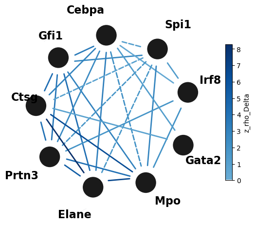
network_from_scenarios turns the result into a network: scenarios 2 and 3 solid, scenario 4 (shared state only) dashed. With one time point there is no direction, so the edges have no arrowheads; colour = z_rho. Which genes to draw depends on the dataset; for LARRY we draw a group of myeloid regulators and the neutrophil-granule genes.
# ============ depends on the dataset (values for LARRY) ============
group = ["Gfi1", "Cebpa", "Spi1", "Irf8", "Gata2", "Mpo", "Elane", "Prtn3", "Ctsg"]
# =================================================================
group = [g for g in group if g in genes]
in_group = result[result["gene_x"].isin(group) & result["gene_y"].isin(group)]
plot_kwargs, edges = network_from_scenarios(in_group, genes=group, weight="z_rho_Delta")   # edge colour = z_rho_Delta
fig, ax = plt.subplots(figsize=(6, 6))
plot_grn(**plot_kwargs, ax=ax, figsize=(8, 8), colorbar_label="z_rho_Delta")
edges.sort_values("weight", key=abs, ascending=False).head(10)
Looks like you are using a tranform that doesn't support FancyArrowPatch, using ax.annotate instead. The arrows might strike through texts. Increasing shrinkA in arrowprops might help.
| source | target | weight | inference_scenario | line_style | directed | z_dag | |
|---|---|---|---|---|---|---|---|
| 25 | Elane | Ctsg | 8.270429 | 3 | solid | False | NaN |
| 21 | Mpo | Elane | 6.751891 | 3 | solid | False | NaN |
| 23 | Mpo | Ctsg | 6.408174 | 3 | solid | False | NaN |
| 24 | Elane | Prtn3 | 5.322118 | 3 | solid | False | NaN |
| 5 | Gfi1 | Elane | 4.364231 | 3 | solid | False | NaN |
| 7 | Gfi1 | Ctsg | 4.350131 | 3 | solid | False | NaN |
| 22 | Mpo | Prtn3 | 4.202826 | 3 | solid | False | NaN |
| 26 | Prtn3 | Ctsg | 4.164198 | 3 | solid | False | NaN |
| 6 | Gfi1 | Prtn3 | 3.859433 | 3 | solid | False | NaN |
| 3 | Gfi1 | Cebpa | 3.581591 | 3 | solid | False | NaN |
6. Several samples
Each sample / time point is scored on its own. Comparing them shows how the balance between regulation and shared states changes, here from day 2 to day 6:
summary, sample_results = [], {}
for value in sorted(obs[sample_column].unique()):
    sample_cells = input_table(adata, value, panel)
    sample_result = infer_with_twinfer(sample_cells, list(sample_cells.columns[1:]),
                                       save_to=sample_folder(value) / "z_scores.csv")
    sample_results[value] = sample_result
    fractions = sample_result["inference_scenario"].value_counts(normalize=True)
    summary.append({sample_column: value, "clones with >= 2 cells": int(sample_result["N_twin_clones"].iloc[0]), "pairs": len(sample_result),
                    **{f"{s} {INFERENCE_SCENARIOS[s]}": round(fractions.get(s, 0.0), 3) for s in (1, 2, 3, 4)}})
summary = pd.DataFrame(summary).set_index(sample_column)
summary
| clones with >= 2 cells | pairs | 1 nothing | 2 regulation | 3 regulation + heterogeneity | 4 heterogeneity | |
|---|---|---|---|---|---|---|
| Time point | ||||||
| 2.0 | 863 | 276 | 0.609 | 0.149 | 0.087 | 0.156 |
| 4.0 | 1674 | 300 | 0.307 | 0.207 | 0.137 | 0.350 |
| 6.0 | 2150 | 276 | 0.130 | 0.127 | 0.395 | 0.348 |
For LARRY, from day 2 to day 6 fewer pairs stay in scenario 1 (day 6 also has more than twice as many clones with two or more cells), and a larger fraction of the pairs is shared within clones (scenarios 3 and 4), as expected when clones commit to a fate.
7. Save the results
Each sample gets its own folder, <sample column>_<value>/ (here Time_point_2/, Time_point_4/, Time_point_6/), with its scores and their settings (already written by save_to in sections 4 and 6), the complete ranked lists by z_rho_s and by z_rho_Delta (not only the top 10) and the number of pairs per inference scenario. The network of section 5 is saved with the sample it was drawn for. The tables that compare the samples (clones per sample, scenarios per sample) are saved in the main folder.
save_result(clones_per_sample.reset_index(), output_dir / "clones_per_sample.csv")
save_result(summary.reset_index(), output_dir / "scenarios_per_sample.csv")
for value, sample_result in sample_results.items():
    folder = sample_folder(value)
    for score, ranked in ranked_edge_lists(sample_result).items():
        save_result(ranked, folder / f"ranked_by_{score}.csv")
    counts = sample_result["inference_scenario"].value_counts().sort_index()
    save_result(pd.DataFrame({"inference_scenario": counts.index, "scenario": [INFERENCE_SCENARIOS[s] for s in counts.index],
                              "pairs": counts.values}), folder / "scenario_counts.csv")
save_result(edges, sample_folder(sample) / "network_edges.csv")
fig.savefig(sample_folder(sample) / "network.pdf", bbox_inches="tight")
sorted(str(p.relative_to(output_dir)) for p in output_dir.rglob("*") if p.is_file())
['Time_point_2/network.pdf',
 'Time_point_2/network_edges.csv',
 'Time_point_2/ranked_by_z_rho_Delta.csv',
 'Time_point_2/ranked_by_z_rho_s.csv',
 'Time_point_2/scenario_counts.csv',
 'Time_point_2/z_scores.csv',
 'Time_point_2/z_scores_settings.json',
 'Time_point_4/ranked_by_z_rho_Delta.csv',
 'Time_point_4/ranked_by_z_rho_s.csv',
 'Time_point_4/scenario_counts.csv',
 'Time_point_4/z_scores.csv',
 'Time_point_4/z_scores_settings.json',
 'Time_point_6/ranked_by_z_rho_Delta.csv',
 'Time_point_6/ranked_by_z_rho_s.csv',
 'Time_point_6/scenario_counts.csv',
 'Time_point_6/z_scores.csv',
 'Time_point_6/z_scores_settings.json',
 'clones_per_sample.csv',
 'scenarios_per_sample.csv']
Notes
Raw 10x output. To build an AnnData-like input from 10x matrices and a barcode / clone table, see
convert_10x_to_twinfer_input.ipynb.Normalisation. Always pass normalised values; the statistics are rank-based, but ranks of raw counts still depend on each cell’s sequencing depth.
One time point at a time. The cross-time direction of the two-time-point tutorial needs sisters measured at two times and is not currently implemented for clone tables.