Simulated twins, two time points: direction of regulation

With twins measured at two time points, TwINFER also infers the direction of regulation: if gene X regulates gene Y, X in one sister at an early time predicts Y in the other sister later, better than Y early predicts X later. This tutorial shows how infer_with_twinfer does this, how to choose the two time points and the gene pairs to test, and how to rank and draw the directed result.

The three z-scores (z_rho, z_rho_s, z_rho_Delta) and the inference scenarios are explained in inference_simulation_one_time_point.ipynb; here they are computed at both time points.

Data. The simulation of the one-time-point tutorial (gene 1 activates gene 2, 6,000 twin pairs, 48 hours after division, simulation_example_output_data/). It has two genes, so there is one gene pair; with more genes, every pair is scored the same way.

1. Setup and data

Results are written to tutorial_output/simulation_two_time_points/, next to this notebook; change output_dir to save them elsewhere. infer_with_twinfer(..., save_to=path) saves its result table (.csv, .csv.gz, .tsv or .parquet) and writes the settings of the call next to it (<name>_settings.json); save_result(table, path) saves any other table the same way.

from pathlib import Path

import matplotlib.pyplot as plt
import numpy as np
import pandas as pd

from twinfer.inference.covariance_decomposition_z_scores import infer_with_twinfer, save_result
from twinfer.inference.ranked_edges import ranked_edge_lists
from twinfer.plotting.network_plots import network_from_scenarios, plot_grn
from twinfer.utils.paths import get_repo_root

output_dir = get_repo_root() / "tutorials" / "tutorial_output" / "simulation_two_time_points"   # where the results are saved (next to this notebook)
table = pd.read_csv(get_repo_root() / "simulation_example_output_data" / "df_rows_0_0_24102026_140638_ncells_6000_A_to_B_04cf9c46.csv")
genes = ["gene_1_mRNA", "gene_2_mRNA"]
print(f"{table['clone_id'].nunique()} twin pairs, time steps {table['time_step'].min()}-{table['time_step'].max()} h")

6000 twin pairs, time steps 0-48 h

2. The design: three groups of clones

Each sister can be measured only once. With two time points t_a < t_b, infer_with_twinfer therefore splits the clones at random (fixed seed; proportions split, default 1:1:2) into

• twin pairs with both sisters measured at t_a (N_a);

• twin pairs with both sisters measured at t_b (N_b);

• a cross group, with one sister measured at t_a and the other at t_b (N_cross).

The covariance z-scores at each time point (suffix _ta for t_a, _tb for t_b) use all cells measured at that time, as for real lineage-tracing data: z_rho uses the twin pairs of that group and the cross-group sister measured then as a singleton (N_clones_ta, N_clones_tb clones in total); z_rho_s and z_rho_Delta need both sisters, so they use the twin pairs of that group.

In the cross group:

• rho_dag_xy: Spearman correlation of X in one sister at t_a with Y in the other sister at t_b; rho_dag_yx the other way round; z_dag = rho_dag × sqrt(N_cross - 1);

• delta = |rho_dag_xy| - |rho_dag_yx|: positive when X → Y, negative when Y → X. The magnitudes are compared, so a repression (negative rho_dag) gets its direction the same way as an activation;

• p_delta: permutation p-value of delta (n_permutations, default 1,000): the cross group is permuted, each null value is built the same way, |rho_dag_xy| - |rho_dag_yx| of the permuted pairs, and p_delta is the share of permutations with |null| ≥ |delta| (+1 in numerator and denominator; the smallest possible value is 1/1001).

As in the paper, the two time points are 1 hour (t_a) and 20 hours (t_b) after division.

result = infer_with_twinfer(table, genes, time_points=[1, 20], save_to=output_dir / "z_scores_1h_20h.csv")
result[["gene_x", "gene_y", "N_a", "N_b", "N_cross", "N_clones_tb", "z_dag_xy", "z_dag_yx", "delta", "p_delta",
        "inference_scenario_ta", "inference_scenario_tb"]]

	gene_x	gene_y	N_a	N_b	N_cross	N_clones_tb	z_dag_xy	z_dag_yx	delta	p_delta	inference_scenario_ta	inference_scenario_tb
0	gene_1_mRNA	gene_2_mRNA	1500	1500	3000	4500	4.800621	-0.883403	0.07153	0.000999	2	2

z_dag_xy is large and z_dag_yx is close to 0: gene 1 at 1 hour predicts gene 2 at 20 hours, not the reverse, so the direction gene 1 → gene 2 is recovered (p_delta at its minimum).

The scenario is reported for both twin groups (inference_scenario_ta, inference_scenario_tb); at 20 hours the pair is in scenario 2, regulation.

3. Other time points

The paper uses 1 and 20 hours. For other systems (other kinetics, other sampling times) the choice may differ: the first time point should be early, when the two sisters are still almost identical, so that one sister at t_a stands for the other; the second late enough for the regulation to act. Scanning the second time point for gene 1 and gene 2 in this simulation, with the first at 1 hour:

rows = []
# for t_a, t_b in [(1, 2), (1, 5), (1, 10), (1, 20), (1, 30), (1, 48), (5, 20), (10, 20)]:   # [2026-10-24 replaced: later first time points removed]
for t_a, t_b in [(1, 2), (1, 5), (1, 10), (1, 20), (1, 30), (1, 48)]:
    r = infer_with_twinfer(table, genes, time_points=[t_a, t_b]).iloc[0]
    rows.append(dict(t_a=t_a, t_b=t_b, z_dag_xy=r.z_dag_xy, z_dag_yx=r.z_dag_yx, delta=r.delta, p_delta=r.p_delta))
time_point_scan = pd.DataFrame(rows)
time_point_scan.round(3)

	t_a	t_b	z_dag_xy	z_dag_yx	delta	p_delta
0	1	2	3.071	0.616	0.045	0.009
1	1	5	5.011	-0.209	0.088	0.001
2	1	10	4.997	-1.224	0.069	0.001
3	1	20	4.801	-0.883	0.072	0.001
4	1	30	5.396	0.421	0.091	0.001
5	1	48	4.311	-1.055	0.059	0.002

With the first time point at 1 hour, the direction is significant for every second time point, already at 2 hours, one hour after the first (there p_delta is larger, 0.009, than from 5 hours on).

With more than two time points in time_points, every pair of them is scored (one row per gene pair and time pair).

4. Many genes: which pairs to test, ranked lists

These two options matter when many genes are scored; with the single pair of this simulation they are only described.

Which pairs get the cross-time correlation. The permutation test makes the cross-time correlation the slowest part. It can be limited with cross_correlation_pairs (the other pairs get NaN in the cross-time columns):

• "all" (default): every gene pair;

• "significant_rho": pairs whose z_rho is significant at t_b;

• "regulation": pairs in scenario 2 or 3 at t_b.

result = infer_with_twinfer(table, genes, time_points=[1, 20], cross_correlation_pairs="regulation")

Ranked lists. With two time points, ranked_edge_lists returns, besides the lists ranked by |z_rho_s| and |z_rho_Delta|, a list ranked by the cross-time correlation z_dag, one row per direction found, written as source → target (z_dag_xy for gene_x → gene_y, z_dag_yx for the reverse). The direction rule (pair_directions, also used by the network of section 5) depends on the scenario at t_b:

• scenario 2 (regulation): each direction is tested on its own, |z_dag| > 1.96 (z_dag_threshold). Both can be listed: mutual regulation;

• scenario 3 (regulation + a shared state): a shared state correlates both directions by itself, so only the difference is used: one direction, the sign of delta, when p_delta < 0.05 (direction_alpha);

• no direction found: one row, the larger |z_dag|, with directed False.

Only pairs with a significant z_rho (at t_b) are ranked, unless significant_rho_only=False. For the pair here:

lists = ranked_edge_lists(result)
lists["z_dag"]

	rank	source	target	directed	z_dag	z_dag_xy	z_dag_yx	delta	p_delta	z_rho	inference_scenario
0	1	gene_1_mRNA	gene_2_mRNA	True	4.800621	4.800621	-0.883403	0.07153	0.000999	1.977758	2

5. Directed network

network_from_scenarios draws scenarios 2 and 3 as solid edges and scenario 4 as dashed edges, using the scenario at t_b (time="tb", default). A solid edge gets its direction by the rule of section 4: in scenario 2 each direction with |z_dag| > 1.96 is drawn (two curved edges for mutual regulation), in scenario 3 one direction when p_delta < 0.05; otherwise it is drawn without direction. Colour = the z_dag of the drawn direction (weight=None, default; z_rho_Delta with one time point); its sign gives an activation arrow or a repression bar.

A mutual repression (toggle switch) usually ends up in scenario 4: its two states are a shared state of the sisters, and both cross-time correlations are then large without telling regulation from the state (two states without regulation look the same), so it is drawn dashed, without direction.

plot_kwargs, edges = network_from_scenarios(result)
plot_kwargs["node_labels"] = ["$g_1$", "$g_2$"]
fig, ax = plt.subplots(figsize=(4.5, 2.5))
plot_grn(**plot_kwargs, ax=ax, fixed_pos={0: (0.2, 0.5), 1: (0.8, 0.5)}, show_colorbar=False, figsize=(8, 8))   # figsize sets line and arrow scale
edges

	source	target	weight	inference_scenario	line_style	directed	z_dag
0	gene_1_mRNA	gene_2_mRNA	4.800621	2	solid	True	4.800621

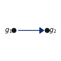
Gene 1 → gene 2 is drawn as a directed edge (activation, positive z_dag). Compare the one-time-point tutorial, where the same pair is drawn without direction.

6. Save the results

The scores at 1 and 20 hours (already written by save_to in section 2), the time-point scan, the ranked lists, the network edges and the network figure.

save_result(time_point_scan, output_dir / "time_point_scan.csv")
for score, ranked in lists.items():
    save_result(ranked, output_dir / f"ranked_by_{score}.csv")
save_result(edges, output_dir / "network_1h_20h_edges.csv")
fig.savefig(output_dir / "network_1h_20h.pdf", bbox_inches="tight")
sorted(p.name for p in output_dir.iterdir())

['network_1h_20h.pdf',
 'network_1h_20h_edges.csv',
 'ranked_by_z_dag.csv',
 'ranked_by_z_rho_Delta.csv',
 'ranked_by_z_rho_s.csv',
 'time_point_scan.csv',
 'z_scores_1h_20h.csv',
 'z_scores_1h_20h_settings.json']

Summary

step	call
covariance z-scores at both times + direction	infer_with_twinfer(table, genes, time_points=[t_a, t_b])
limit the cross-time correlation	cross_correlation_pairs="significant_rho" or "regulation"
ranked lists, including the cross-time correlation	ranked_edge_lists(result)
directed network	plot_grn(**network_from_scenarios(result)[0])
save the scores	infer_with_twinfer(..., save_to="scores.csv"), or save_result(table, "table.csv")

For real lineage-tracing data (clones instead of exact twins), see inference_real_data_lineage_tracing.ipynb; there, each time point is scored on its own.