Simulated twins, one time point: covariance decomposition and inference scenarios

This tutorial shows how to score a pair of genes with infer_with_twinfer when twins are measured at one time point, read the three z-scores and the inference scenario it reports, and draw the result as a network. The direction of regulation needs two time points: see inference_simulation_two_time_points.ipynb.

What TwINFER uses. Sister cells (“twins”) come from the same mother cell. Right after division they share their molecules and the cell state they inherited; with time, each sister’s expression drifts away from the other’s. Because of this, the correlation of two genes across cells can be split into a part the twins share and a part that differs between twins. The two parts tell apart two reasons why two genes are correlated:

• regulation: X acts on Y in every cell, so the correlation shows up in the twin differences too;

• heterogeneity: cells sit in different states (for example two cell types) that set both genes. Twins sit in the same state, so the correlation is shared by twins and is absent from their differences.

The three z-scores (one gene pair, N twin pairs):

z-score	measures	significant when
z_rho	the expression correlation of X and Y over all cells (Spearman)	|z| > 1.96
z_rho_s	the twin-shared part: X in one sister against Y in the other sister	|z| > 2.326
z_rho_Delta	the correlation of the twin differences (X in sister 1 minus sister 2, the same for Y)	|z| > 1.96

All three are analytic (no shuffling) and use N = the number of twin pairs. For real lineage-tracing data (clones of any size, many gene pairs, Benjamini-Hochberg correction), see inference_real_data_lineage_tracing.ipynb.

The four inference scenarios follow from these z-scores:

scenario	z_rho	z_rho_s	z_rho_Delta	reading
1 nothing	not significant			no correlation
2 regulation	significant	not significant		correlation not shared by twins
3 regulation + heterogeneity	significant	significant	significant	shared part and a twin-difference part
4 heterogeneity	significant	significant	not significant	correlation only through a shared state

Data used here. A simulated two-gene network in which gene 1 activates gene 2 (A → B), with 6,000 twin pairs followed for 48 hours after division. The file ships with the repository in simulation_example_output_data/.

1. Setup

Install the package once from the repository root (pip install -e package/, see the README). Then:

Results are written to tutorial_output/simulation_one_time_point/, next to this notebook; change output_dir to save them elsewhere. infer_with_twinfer(..., save_to=path) saves its result table (.csv, .csv.gz, .tsv or .parquet) and writes the settings of the call next to it (<name>_settings.json); save_result(table, path) saves any other table the same way.

from pathlib import Path

import matplotlib.pyplot as plt
import numpy as np
import pandas as pd

from twinfer.inference.covariance_decomposition_z_scores import (
    INFERENCE_SCENARIOS,
    classify_inference_scenario,
    infer_with_twinfer,
    save_result,
)
from twinfer.plotting.network_plots import network_from_scenarios, plot_grn
from twinfer.utils.paths import get_repo_root

output_dir = get_repo_root() / "tutorials" / "tutorial_output" / "simulation_one_time_point"   # where the results are saved (next to this notebook)
data_file = get_repo_root() / "simulation_example_output_data" / "df_rows_0_0_24102026_140638_ncells_6000_A_to_B_04cf9c46.csv"

2. The input table

infer_with_twinfer reads a long table with one row per cell and time point:

• clone_id: the twin pair (the mother cell);

• replicate: 1 or 2, which sister;

• time_step: hours after division;

• one column per measured quantity. The simulation also stores protein counts; TwINFER uses the mRNA columns, as in real data.

table = pd.read_csv(data_file)
print(f"{table['clone_id'].nunique()} twin pairs, time steps {table['time_step'].min()}-{table['time_step'].max()} h")
table.head()

6000 twin pairs, time steps 0-48 h

	cell_id	time_step	gene_1_A	gene_1_I	gene_1_mRNA	gene_1_protein	gene_2_A	gene_2_I	gene_2_mRNA	gene_2_protein	replicate	clone_id
0	0	0	0	1	1	29434	1	0	3	137518	1	0
1	0	1	0	1	0	29250	0	1	4	137216	1	0
2	0	2	0	1	0	28802	0	1	2	137106	1	0
3	0	3	0	1	0	28366	0	1	2	136148	1	0
4	0	4	0	1	0	27921	0	1	1	134610	1	0

3. Score the gene pair at one time point

We use the mRNA counts 20 hours after division. With one time point in time_points, the function compares the two sisters of every twin pair at that time. save_to writes the result to a file.

genes = ["gene_1_mRNA", "gene_2_mRNA"]
result = infer_with_twinfer(table, genes, time_points=[20], save_to=output_dir / "z_scores_20h.csv")
result[["gene_x", "gene_y", "N", "z_rho", "z_rho_s", "z_rho_Delta", "inference_scenario"]]

	gene_x	gene_y	N	z_rho	z_rho_s	z_rho_Delta	inference_scenario
0	gene_1_mRNA	gene_2_mRNA	6000	4.335645	-0.908895	3.819923	2

z_rho and z_rho_Delta are significant, z_rho_s is not. The pair is called scenario 2, regulation:

• z_rho is large: the two genes are correlated;

• z_rho_s (-0.9) is below 2.326 in absolute value: what sister 1 expresses of gene 1 tells little about what sister 2 expresses of gene 2, so the correlation is not carried by a shared state;

• z_rho_Delta is large: when one sister has more gene 1 than its twin, it also has more gene 2. Regulation acts inside each cell.

The table holds the quantities the z-scores are built from. S is the Spearman correlation over all cells. C is its twin-shared part and U = S - C the unshared part. h_x, h_y are the sister correlations of each gene (how alike the twins are). z_rho splits exactly into a shared and an unshared contribution, z_rho = A_s + A_u:

row = result.iloc[0]
print(f"S = {row.S:.4f} = C + U = {row.C:.4f} + {row.U:.4f}")
print(f"z_rho = {row.z_rho:.3f} = A_s + A_u = {row.A_s:.3f} + {row.A_u:.3f}")
print(f"sister correlations: h_x = {row.h_x:.3f}, h_y = {row.h_y:.3f}")

S = 0.0396 = C + U = -0.0083 + 0.0479
z_rho = 4.336 = A_s + A_u = -0.910 + 5.245
sister correlations: h_x = 0.005, h_y = 0.053

The scenario can also be computed from any three z-scores with classify_inference_scenario (thresholds can be changed with thresholds=(z_rho, z_rho_s, z_rho_Delta)):

scenario = classify_inference_scenario(row.z_rho, row.z_rho_s, row.z_rho_Delta)[0]
print("scenario", scenario, INFERENCE_SCENARIOS[scenario])

scenario 2 regulation

4. How many twin pairs are needed

For a fixed correlation, the z-scores grow with the square root of the number of twin pairs. Scoring one random subset of twin pairs per size at 20 hours:

rng = np.random.default_rng(0)
twin_pairs = table["clone_id"].unique()          # clone_id = twin pair
rows = []
for n in [100, 250, 500, 1000, 3000, 6000]:
    chosen = rng.choice(twin_pairs, size=n, replace=False)
    rows.append(infer_with_twinfer(table[table["clone_id"].isin(chosen)], genes, time_points=[20]))
subsets = pd.concat(rows, ignore_index=True)
subsets[["N", "z_rho", "z_rho_s", "z_rho_Delta", "inference_scenario"]]

	N	z_rho	z_rho_s	z_rho_Delta	inference_scenario
0	100	0.853473	0.248670	0.471304	1
1	250	0.339194	-0.746497	0.768268	1
2	500	1.128331	-0.663825	1.272831	1
3	1000	2.785662	-0.136306	2.106277	2
4	3000	3.103083	-0.647381	2.728443	2
5	6000	4.335645	-0.908895	3.819923	2

The correlation in this example is weak (Spearman 0.04 at 20 hours), so with fewer than about 1,000 twin pairs it is not reliably detected; each subset is a single random draw, so the small sizes scatter.

5. Draw the result as a network

network_from_scenarios turns the result table into the inputs of plot_grn:

• scenario 2 (regulation): solid edge, colour = z_rho_Delta;

• scenario 3 (regulation + heterogeneity): blue dashed edge;

• scenario 4 (heterogeneity, a shared state): grey dashed edge;

• scenario 1: no edge.

With one time point there is no direction, so edges are drawn without arrowheads (with two time points they get one, see the next tutorial). \(g_1\) and \(g_2\) below are gene 1 and gene 2, scored 20 hours after division (the result of section 3):

labels = {"gene_1_mRNA": "$g_1$", "gene_2_mRNA": "$g_2$"}
positions = {0: (0.2, 0.5), 1: (0.8, 0.5)}

plot_kwargs, edges = network_from_scenarios(
    result,
    solid_scenarios=(2,),                            # regulation: solid, coloured by z_rho_Delta
    dashed_scenarios=(3, 4),                         # regulation + heterogeneity, heterogeneity: dashed
    scenario_colors={3: "tab:blue", 4: "grey"},
)
plot_kwargs["node_labels"] = [labels[g] for g in plot_kwargs["node_labels"]]
fig, ax = plt.subplots(figsize=(4.5, 2.5))
plot_grn(**plot_kwargs, ax=ax, fixed_pos=positions, show_colorbar=False, figsize=(8, 8))   # figsize sets line scale
edges

	source	target	weight	inference_scenario	line_style	directed	z_dag
0	gene_1_mRNA	gene_2_mRNA	3.819923	2	solid	False	NaN

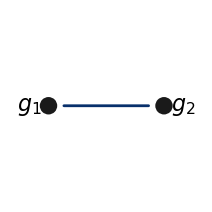
The pair is called regulation (scenario 2), so the edge is solid. The same calls work for any number of genes: pass all gene columns to infer_with_twinfer and the whole result table to network_from_scenarios. plot_grn(**plot_kwargs) draws the nodes on a circle when fixed_pos is not given.

6. Save the results

Everything this tutorial computed: the scores at 20 hours (already written by save_to in section 3), the scores of the twin-pair subsets, the network edges and the network figure.

save_result(subsets, output_dir / "z_scores_20h_twin_pair_subsets.csv")
save_result(edges, output_dir / "network_20h_edges.csv")
fig.savefig(output_dir / "network_20h.pdf", bbox_inches="tight")
sorted(p.name for p in output_dir.iterdir())

['network_20h.pdf',
 'network_20h_edges.csv',
 'z_scores_20h.csv',
 'z_scores_20h_settings.json',
 'z_scores_20h_twin_pair_subsets.csv']

Summary

step	call
score gene pairs at one time point	infer_with_twinfer(table, genes, time_points=[t])
add the direction (next tutorial)	infer_with_twinfer(table, genes, time_points=[t_a, t_b])
scenario from z-scores	classify_inference_scenario(z_rho, z_rho_s, z_rho_Delta)
network figure	plot_grn(**network_from_scenarios(result)[0])
save the scores	infer_with_twinfer(..., save_to="scores.csv"), or save_result(table, "table.csv")

Next: inference_simulation_two_time_points.ipynb (direction of regulation) and inference_real_data_lineage_tracing.ipynb (real data). The analyses of the paper that use these functions are in paper_analysis/ (for example heterogeneity_vs_regulation/ scores single-state, two-state and drifting simulations the same way).